26 Dec Using GPE3 to Improve Geolocation Estimates
Using light to estimate your position on the globe is not new; mariners used celestial navigation for centuries before modern technologies like LORAN (developed in the 1940s) and GPS (developed in the 1970s) became available. Using light to estimate animals’ locations is not new either, and Wildlife Computers was at the forefront of implementing geolocation algorithms on electronic tags as early as 1989.
What is new is the growing cadre of smart researchers figuring out the best ways to improve geolocation estimates using robust statistical models. Estimates are improved by using all kinds of complementary environmental data, such as tidal heights, magnetic fields, temperatures at particular depths, and by applying barriers to prevent movement on land. Newer models produce statistical measures of uncertainty and many can accommodate prior information in a Bayesian framework. Wildlife Computers evolved along with the scientific community. Who, besides me, remembers when we manually stepped through each set of light-level data, eliminated outlying points, and tried to get the perfect curve shape and low Mean Square Errors? Then most of us took the output and ran it through some kind of smoother, or tried to match temperatures to satellite data, often deleting locations around the equinoxes.
Since 2015, Wildlife Computers has provided GPE3 as a way to obtain light-based geolocation estimates of movements from the light data collected by our tags. GPE3 is a discretized (i.e. progressing in small time steps) Hidden Markov Model (a type of state-space model) that uses observations of light, sea surface temperature, maximum swimming depth, and any known locations that you may have from different types of data collections such as Argos, GPS locations, acoustic tags, or even visual observations. The hidden states in the model are the possible locations where the animal may have been at any given time. The model is fully integrated and incorporates a movement model based on a speed parameter chosen by the researcher and an observation model based on all the light, SST, depth, and known location data. The output is a grid of locations and the associated probability that the animal was in each grid cell at each time step. You can run the GPE3 model in the Location Processing section of the Wildlife Computers Data Portal. For those of you who wish to dig into the mathematical details, the model is based on the methods of Pedersen et al. (2011).
Key benefits of using GPE3 are that it is simple to run using our Data Portal, provides statistically robust estimates of the probable locations of your animal, is relatively fast, and runs on our servers thus doesn’t tie up your computer’s resources.
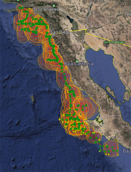 The figure shows the most probable locations and the 50%, 95% and 99% probability contours for a fish off the coast of California and Baja California based on light, SST and Fastloc® GPS data. Data courtesy of Heidi Dewar, NOAA Fisheries.
Undoubtably, the scientific community is looking for better and better ways to derive light-based geolocation estimates. That’s what scientists do! That may mean finding a better way to sample the light data, or a better model to estimate positions and their uncertainty or perhaps using unique types of observation data to complement the light data. Wildlife Computers is keeping an eye out for better solutions to keep up with progress. For now, we are happy with GPE3 and hope you are too!
Below are a few tips for running GPE3. For more information on location processing see the Location Processing User Guide. If you run into problems, feel free to email me.
Speed—the parameter that has the greatest influence on your results is the speed parameter. The movement model assumes that the inputted speed is on the high side (about one standard deviation above the mean) of typical sustained horizontal swimming speeds. Typical swimming speeds could be derived from the literature for your species or similar species, from prior observations or tracking studies, or based on expert knowledge. We usually find that inputting a speed around 1.5 times or twice the average sustained swimming speed works well. If the model runs to zero, the most likely reason is that the speed parameter is too low. Try bumping up the speed parameter, within reason, and see if that helps.
Location on Land—you may encounter an error indicating that locations are on land. That could happen when any of your known locations (deployment start or end locations, Fastloc, Argos or other observations) are very close to shore. The resolution of the model is 0.25 x 0.25 degrees, and if a large part of a grid cell is on land, that grid cell will be excluded from the state space of possible locations. The solution is to bump your known locations a tad (usually 0.125 degrees is enough) offshore.
Suzy Kohin joined Wildlife Computers in June 2018. Kohin holds a bachelor’s degree in Math and French from Washington University in St. Louis and a Ph.D. in Biology from UC Santa Cruz. Kohin’s research includes analyzing and applying electronic tagging data to questions regarding habitat-use, foraging ecology, population structure, survivorship, and fisheries management. At Wildlife Computers, Kohin interacts with researchers about their needs and helps investigate novel ways that tagging technologies can advance science and conservation efforts. Suzy has published extensively in fisheries, quantitative ecology, and physiology. You can find a full list of her publications here.